[BA03. On-Time Risk: Appendix 1] Anatomy of the EXA Bayesian Engine: Mixture Distributions and Observational Deviation

This is the first article in a technical explanation series identifying the operating principles of the EXA engine, which played a major role in the novel-style series 'BA03 On-Time Material Inbound: Bayesian MCMC'.

Since this series covers Mixture Distributions and MCMC (Markov Chain Monte Carlo) Gibbs Sampling—which are advanced techniques in Bayesian inference—the content may be deep and the calculation process somewhat complex. Therefore, we intend to approach this in a detailed, step-by-step manner to make it as digestible as possible, and it is expected to be a fairly long journey.

We recommend reading the original novel first to understand the overall context. Furthermore, as Bayesian theory expands its concepts incrementally, reviewing the episodes and mathematical explanations of BA01 and BA02 beforehand will be much more helpful in grasping this content. The preceding mathematical concepts and logic are being carried forward.

1. Definition of Data: Observation Deviation

To mathematically model the core issue addressed in the novel, 'On-Time (punctual arrival),' we must first define the data. To this end, we generate sample observation data on a daily basis as follows.

We can view this set of observed delay days, $D$, as a single Vector, and each delay value within it (-2, -1, 0 ...) becomes an Element (or component) constituting this vector.

Here, each individual data element $d_i$ is defined as follows:

The meaning of this formula is very intuitive:

• $d_i = 0$: The case where the promise was kept exactly (On-Time)

• $d_i > 0$: Cases delayed beyond the plan (e.g., +5 means a 5-day delay)

• $d_i < 0$: Cases arriving earlier than planned (Early Delivery)

This model of Delay Days can be applied to measure various bottlenecks in the business field:

• Material inbound and supplier work delays (Lead Time Delay)

• Transportation and logistics delays (Transportation Delay)

• Production line process delays (Production Delay)

The size (dimension) of the vector data is determined by the scale of the business. If there are 100 observed transaction records, it will be a vector consisting of 100 elements; if there are 300 records, it will be 300 elements.

In this series, to clearly anatomize the operating principles of the EXA engine, we use the seven 'Toy Data' points defined earlier as an example. While hundreds or thousands of data points are realistic, they have limitations in intuitively demonstrating complex calculation processes.

Of course, when applied to actual fields, data must be managed with granularity according to decision-making purposes, such as "Supplier + Item + Transport Mode + Destination" or production's "Line + Product," allowing for accurate capture of overall SCM risks.

2. Visualization of Data: Two Peaks

Now, let's visualize our toy data (Vector $D$). Let's check how the seven elements are arranged on the graph.

 

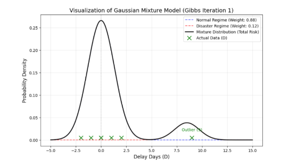
What does real-world data look like? Below is a histogram showing 200 material purchase transaction records (for a specific item from a specific supplier) of an actual company.

 

Interesting similarities are discovered. Our toy data is scattered around the normal state (0) while simultaneously forming a separate peak representing a delayed state (9). Actual corporate data is also divided into a peak centered around the normal lead time average of 23 days and another, albeit weaker, peak centered around the delayed state of 33 days.

Most delay day data takes the form of having two peaks like this. In actual data, three or more peaks may occasionally appear. However, rather than modeling every peak in the data individually, we compress it into a 2-regime (Normal/Delayed) model to match the structure where decision-making is actually executed (Normal Operations vs. Abnormal Response).

This is not a simple reduction of reality. It is an aspect of Operational Design that reduces uncertainty, stabilizes judgment, and makes execution consistent. Detailed patterns (such as minor delays) can be expanded when necessary, but the basic engine is most robust when defined by two states (Regimes): 'Normal' and 'Delayed.'

3. Statistical Assumption: Validity of the Normal Distribution

Here, we establish an important statistical assumption: "Delay day data follows a Normal Distribution scattered in a bell shape around the mean."

Why the Normal Distribution?

Some might ask, "Does reality really follow a normal distribution like a textbook?" However, according to the Central Limit Theorem of statistics, the resulting values produced by the combination of various independent variables (worker's condition, weather, traffic situations, minute mechanical errors, etc.) converge to a normal distribution if the sample size is sufficient. In other words, modeling the uncertainty of processes and logistics as a normal distribution is the most mathematically valid and rational approach.

4. Conclusion and Next Steps

Ultimately, the graph we are looking at is a combination of a 'Normal State Normal Distribution' and a 'Delayed State Normal Distribution.' This is the reality of the Mixture Distribution that the EXA engine in the novel intends to interpret.

[Conclusion of Part 1] The data we observed, namely the Likelihood function, is a mixture distribution composed of two individual normal distributions.

The primary goal is to find the On-Time Risk, that is, the probability that a delay may occur, from this observation data composed of mixture distributions using Bayesian inference.

To this end, the next article [Appendix 2] will design a specific mathematical model to solve the likelihood function composed of mixture distributions through a Bayesian approach.