- Published on
BA026. Consensus of the Particles — The Math of MCMC Ensembles and Cross-Validation
In BA025, Grid Search scanned 3,240 grid points to find the optimal candidate parameters that maximize Youden's J. But one crucial question remains:
"Can that optimal value really be trusted?"
Grid Search provides only a Point Estimate. It said T(Discovery)=0.22 is optimal, but does the result change completely if you shift to 0.21 or 0.23? Or does it stay similar? Without that answer, a sales leader cannot trust the number.
This post unpacks the mathematical principles behind Auto-Tuner's second pillar — MCMC Ensemble Sampling — and its third pillar — Cross-Validation.
Part I. MCMC Ensemble Sampling
1. Posterior Distribution: The Answer Is Not a 'Point' but a 'Landscape'
The core philosophy of Bayesian inference is that a parameter's optimal value is not a single point but a Probability Distribution.
If Grid Search answered "T(Discovery)=0.22," what we truly want to know from a Bayesian perspective is:
That is, the Posterior Distribution — "the complete landscape of probabilities for every possible value of parameter θ, after observing the data."
The peak (Mode) of this posterior is the optimal point, and the width of the peak represents the magnitude of uncertainty. A sharp peak means "this value is certain"; a wide one means "many values are similarly good."
The problem is that computing this posterior mathematically is impossible in most real-world problems. The denominator P(Data) — the Evidence — requires a high-dimensional integral:
An integral over 6 dimensions — 5 T-values and 1 k-value. No analytical solution exists.
This is where MCMC enters.
2. What Is MCMC?
For readers encountering MCMC for the first time, let's break down the name.
MCMC = Markov Chain + Monte CarloThe name combines two mathematical ideas.
Monte Carlo — Named after the famous casino city in Monaco. The core idea: "If exact computation is impossible, run random simulations thousands of times to approximate the answer." For example, to compute the area of a circle without a formula: scatter thousands of random points on a square, count how many fall inside the circle, and you can estimate π. That's the Monte Carlo method.
Markov Chain — Named after Russian mathematician Andrey Markov. A stochastic path where "the next state depends only on the current state, not on the history of past states" (memorylessness). Think of a drunk person stumbling through alleyways: the direction of the next step depends only on where they're standing now, not where they started.
Combining them into MCMC: "A method that wanders randomly through parameter space following Markov Chain rules (probabilistically selecting the next position from the current one), and estimates the posterior distribution from the distribution of that trajectory."
Why is such a method necessary? As shown earlier, directly computing the posterior P(θ|Data) requires the high-dimensional integral of the denominator P(Data). This integral is mathematically unsolvable for most real-world problems. MCMC is the most powerful tool in modern computational statistics — one that sidesteps this integral while still revealing the shape of the posterior distribution.
Since the 1990s, with the explosive growth of computing power, MCMC has become a standard tool across nearly every field — physics, astronomy, genetics, financial engineering. Auto-Tuner's use of MCMC for sales parameter optimization is the application of this proven methodology to the business domain.
MCMC, Deep Learning, Reinforcement Learning — Same Root, Different Branches
MCMC may feel unfamiliar, but it shares remarkably deep connections with today's core AI technologies.
Connection to Deep Learning — "The journey to find optimal parameters"Consider the training process in deep learning. A neural network has millions of weights, and SGD (Stochastic Gradient Descent) descends the slope of the loss function to find optimal weights. MCMC does essentially the same thing — finding optimal points in parameter space. The difference is methodology. SGD is a mountaineer following the "steepest downhill path"; MCMC is an expedition team "wandering probabilistically to map the entire terrain." SGD finds a single optimum quickly but knows nothing about the uncertainty around it. MCMC is slower but tells you "how certain this answer is." For Auto-Tuner, the latter matters more — because a sales leader needs to hear "the optimum is 0.22, and the safe range is 0.19–0.25."
Connection to Reinforcement Learning — "Balancing exploration and exploitation"The core dilemma of Reinforcement Learning (RL) is Exploration vs. Exploitation — "try new actions (exploration) or repeat the best-known action (exploitation)." MCMC's accept/reject mechanism solves exactly this dilemma. If the new position (θ') has a higher posterior probability than the current position (θₜ), it always moves (exploitation); even if it's lower, it moves with a certain probability (exploration). This balance lets MCMC avoid being trapped at a Local Optimum and navigate toward the Global Optimum. RL's ε-greedy strategy and Policy Gradient methods stand on fundamentally the same principle.
Common DNA of the three technologiesDeep Learning, Reinforcement Learning, MCMC — all three share a common DNA: "methods for probabilistically searching for optimal solutions in high-dimensional spaces." ChatGPT optimizing billions of parameters and Auto-Tuner optimizing 6 sales parameters differ only in scale; the mathematical thinking belongs to the same family.
Now let's see specifically how MCMC works.
3. Mathematical Procedure of MCMC
- Choose an initial point: Start at an arbitrary position θ₀ in parameter space.
- Proposal: Propose a new position θ' from the current position θₜ.
- Accept/Reject: Compute the acceptance probability α:
Why is this formula so powerful? Let's trace where the acceptance probability α actually comes from.
What we really want to compare is the ratio of "posterior probability at θ'" to "posterior probability at θₜ":
Substituting Bayes' theorem for each:
Here's where the key insight emerges. The same P(Data) appears in both numerator and denominator. Simplifying the fraction of fractions:
P(Data) cancels out completely. This is MCMC's core trick. The P(Data) that required a 6-dimensional integral never needs to be computed at all. Because we only need to "compare" the posterior probabilities at two points, the denominator common to both sides naturally cancels.
As a result, the acceptance probability can be calculated using only the Likelihood and the Prior — both of which are easy to compute.
- Move: Accept θ' with probability α and move there. If rejected, stay at θₜ.
- Repeat: Iterate thousands to tens of thousands of times.
The chain produced by this process — θ₀, θ₁, θ₂, ..., θₙ — converges in distribution to the posterior after sufficient iterations. This is guaranteed by the Ergodic Theorem.
4. Emcee: The Affine-Invariant Ensemble Sampler
Auto-Tuner uses not a standard MCMC but Emcee (Goodman & Weare, 2010), a specialized ensemble sampler. There's a reason.
Problems with Standard MCMC
Traditional MCMC (e.g., Metropolis-Hastings) explores the posterior with a single chain. Two problems arise:
Problem 1 — Correlated Parameters: If T(Qualification) and T(Solution-Fit) are highly correlated, the posterior forms an elongated ellipse along the diagonal. A single chain cannot traverse this ellipse efficiently and explores slowly like a random walk.
Problem 2 — Multimodality: If the posterior has multiple peaks, a single chain may become trapped in one peak and fail to discover the others.
Emcee's Solution: Ensembles
Instead of a single chain, Emcee releases hundreds of walkers simultaneously into parameter space. Auto-Tuner uses 256 walkers.
The movement rule for each walker is key. When walker j moves, it references the current position of another walker k:
Where z is drawn from:
a is a tuning parameter (default 2.0).
Why "Affine Invariant"?
The most important property of this algorithm is affine invariance. The algorithm's performance does not change under linear transformations (rotation, scaling, shearing) of the parameter space.
In business terms: T(Discovery) ranges from 0.01–0.10 while k ranges from 0.5–2.5 — parameters with completely different scales can be explored efficiently without separate standardization.
This is the decisive reason Auto-Tuner chose Emcee. Sales parameters have different scales and correlation structures across dimensions, and Emcee operates most efficiently on such irregular terrain.
The Significance of 256 Walkers
The reason for 256 walkers is based on an empirical rule:
Auto-Tuner explores 6 dimensions (5 T-values + 1 k), requiring a minimum of 12, but uses 256 for thorough posterior exploration. More walkers mean faster convergence, but there is a computation trade-off.
5. Convergence Diagnostics: R̂ (R-hat)
Before trusting MCMC results, one thing must be verified: Has the chain truly converged to the posterior?
A chain still near its starting position may show only a fragment of the posterior. The standard tool for detecting this is the Gelman-Rubin R̂ (R-hat) statistic.
The Math of R̂
Given multiple independent chains (C₁, C₂, ..., Cₘ):
Between-chain variance (B):
Within-chain variance (W):
R̂ calculation:
Interpretation
- R̂ ≈ 1.00: All chains have converged to the same distribution. ✅ Results are trustworthy.
- R̂ > 1.05: Inconsistency between chains. ⚠️ More iterations needed.
- R̂ > 1.10: Serious non-convergence. ❌ Results should not be used.
Business Analogy
256 explorers (walkers) were released from different starting points. After sufficient time:
- R̂ ≈ 1.0: All 256 reached the same conclusion: "The optimum is in this range." → Consensus achieved.
- R̂ > 1.1: Some explorers are still wandering elsewhere. → No consensus. More exploration time needed.
Auto-Tuner sets R̂ < 1.05 as a mandatory condition. If this is not met, it automatically increases the number of sampling iterations and retries.
6. HDI 95% Credible Interval
From the converged posterior samples, the HDI (Highest Density Interval) is extracted.
HDI vs. Standard Confidence Interval
A standard 95% Confidence Interval (CI) trims 2.5% from each tail. For symmetric distributions, HDI and CI are identical, but for asymmetric distributions, they differ.
HDI is "the narrowest interval from the posterior distribution that contains 95% of the total probability, comprised of regions with the highest probability density."
Where c is the density threshold that makes the region's probability exactly 0.95.
Business Implications
Revisit the result the system showed in BA024:
T(Discovery): 0.19 ~ 0.25 (Optimal: 0.22)
This is the HDI. It means: "Based on 106 deals, the optimal T(Discovery) is 0.22, and performance is maintained with 95% probability anywhere between 0.19 and 0.25."
This is overwhelmingly more useful information than Grid Search's point estimate of "0.22."
If you tell a sales leader "Set T(Discovery) to 0.22," they'll suspect "Does it have to be exactly 0.22? What if I use 0.20?" But if you say "Anywhere within 0.19–0.25 is safe, backed by data," conviction that leads to action emerges.
Part II. Cross-Validation and Diagnostics
7. 5-Fold Cross-Validation: Testing the Future
The optimal parameters derived by Grid Search and MCMC work perfectly on historical data. But the real question is:
"Will these parameters work on future deals that haven't been seen yet?"
This is the core of the Overfitting problem.
The Overfitting Analogy
A student who obtained the exam answers in advance scored 100. To know if they truly understand physics, they need to take a different exam.
Likewise, whether parameters optimized on 106 historical deals are accurate for the 107th future deal can only be assessed by evaluating with data that were "unseen."
The Mathematical Procedure of 5-Fold
Step 1. Randomly partition 106 deals into 5 equal-sized Folds.
| Fold 1 | Fold 2 | Fold 3 | Fold 4 | Fold 5 |
|---|---|---|---|---|
| 21 deals | 21 deals | 22 deals | 21 deals | 21 deals |
Step 2. First iteration: Train on Folds 2–5 (85 deals), test on Fold 1 (21 deals).
Step 3. Second iteration: Train on Folds 1, 3–5 (85 deals), test on Fold 2 (21 deals).
Repeat 5 times.
Step 4. Final cross-validation score:
Interpretation Criteria
- High average J with small standard deviation → Parameters are stable. Not overfitting.
- High average J but large standard deviation → Unstable parameters fitting only specific data. Overfitting suspected.
- Cross-validation J significantly lower than full-data J → Overfitting confirmed.
BA024 Results
Average accuracy: 75.5% (±1.2%)
The difference between full-data J=0.74 and cross-validation average J≈0.73 is only 0.01. And inter-fold standard deviation is 1.2 percentage points. This is strong evidence that the parameters are not overfitting to historical data and similar performance can be expected on future deals.
8. Signal Lift Analysis: Which Signals Truly Matter?
A powerful analysis generated as a byproduct of Auto-Tuner's cross-validation phase is Signal Lift.
Definition of Lift
Compare the win rate of deals where signal S was observed versus those where it was not:
Interpretation
- Lift > 1: Observing signal S increases win probability. → Meaningful signal.
- Lift ≈ 1: Signal S has no impact on winning. → Noise.
- Lift < 1: Observing signal S actually decreases win probability. → Inverse signal.
Business Diagnostics
What the VP of Sales discovered in BA024:
| Signal | Lift | Interpretation |
|---|---|---|
| Competitor info shared | +3.2 | When the customer reveals competitor cards, win probability ×3.2 ↑ |
| MSA review initiated | +2.8 | When legal begins contract review, near-certain stage |
| Budget approval confirmed | +1.4 | Less decisive for winning than expected (reorg risk) |
| Meeting attendance increase | +0.3 | Effectively noise — spectator effect |
Signal Lift enables redesigning the sales strategy. Energy spent on "getting lots of people to meetings" can be redirected to "building relationships that naturally elicit competitor information."
9. Mismatch Alert: Gap Between Settings and Data
Auto-Tuner's final diagnostic function is the Mismatch Alert.
Principle
It compares each signal's user-set Impact Score against the actual contribution observed in data (based on Signal Lift):
- Ratio ≈ 1.0: User intuition matches data. ✅
- Ratio > 1.5: User overestimates the signal. ⚠️ May cause False Positives.
- Ratio < 0.67: User underestimates the signal. ⚠️ May cause False Negatives.
BA024 Example
Signal "Budget Approval" has a current Impact Score (2.5) inconsistent with the data-recommended value (1.7).
Mismatch Ratio = 2.5 / 1.7 = 1.47. Approaching the threshold (1.5), triggering a warning.
Business Implications
Mismatch Alert is a mechanism for detecting Organizational Bias.
An old assumption may persist: "In our company, once the budget is approved, it's practically done." But the past year's data says: "20% of deals still fell through after budget approval."
Mismatch Alert makes these 'unfelt biases' visible through data. It's not criticism — it's an early warning that the environment has changed.
10. The Full Pipeline: Three Pillars Working Together
Auto-Tuner's three pillars are not independent. They form a single sequential pipeline.
Grid Search → "Among all possible combinations, find the candidate with the highest J."
MCMC → "Determine how certain that candidate is, what alternatives exist, and reveal the entire distribution."
Cross-Validation → "Test whether these results work only on the past, or will hold for the future as well."
Using a medical analogy for each stage:
| Stage | Medical Analogy | Role |
|---|---|---|
| Grid Search | Full-body scan (CT) | Rough identification of problem area |
| MCMC | Precision scan (MRI) | Detailed mapping of that area |
| Cross-Validation | Clinical trial | Verify if the treatment works on other patients |
Only after passing all three stages does Auto-Tuner display the final proposal: "Would you like to apply these parameters?" If any stage falls short — R̂ > 1.05, or cross-validation variance is excessive — it raises a warning and recommends collecting more data.
11. Epilogue: An Engine Tuned by Data
In BA024, the VP of Sales ran Auto-Tuner for the first time and said:
"Six months ago, I tuned the engine. Starting today, data tunes the engine."
This is not mere sentiment. It is a mathematically precise statement.
- Past: Parameter θ set by human experience P(θ). → Inference trapped in the prior.
- Present: When data D is observed, θ is updated to P(θ|D). → Inference based on the posterior.
Auto-Tuner is the Meta-layer that enables the sales engine to perform Bayesian inference on its own parameters.
Just as the engine infers the win probability of deals, Auto-Tuner infers the engine's own configuration values. And as deals accumulate, inference becomes more precise. 500 deals provide a narrower HDI than 100 deals; 1,000 deals narrower still.
This is the essence of Auto-Tuner — a self-evolving inference system that becomes more precise over time.
Sales is no longer the domain of gut feeling. The volume of data is the engine's precision, and precision is the organization's competitive edge. Auto-Tuner is the accelerator on that journey.
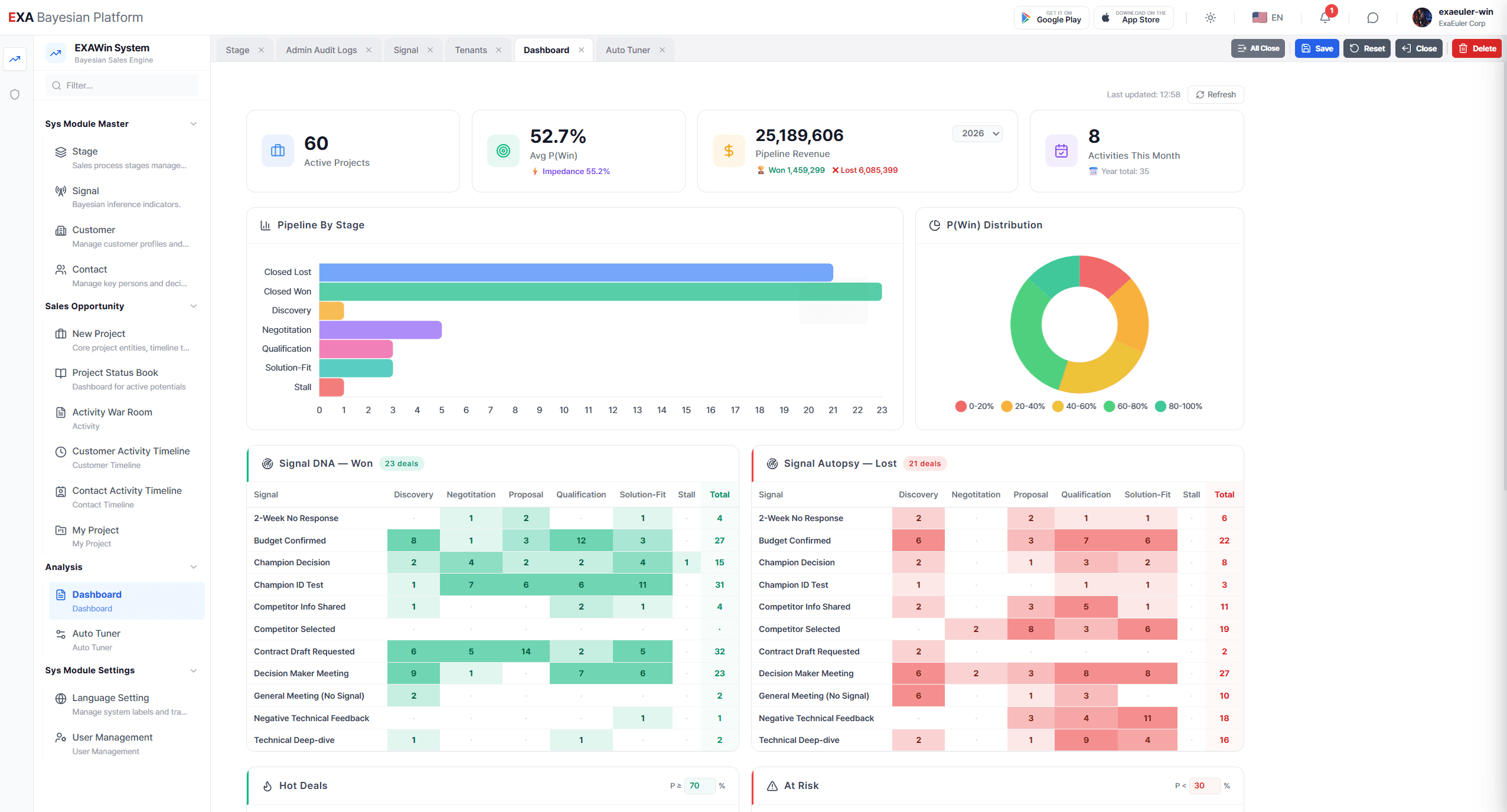
Bayesian EXAWin-Rate Forecaster
Precisely predict sales success by real-time Bayesian updates of subtle signals from every negotiation. With EXAWin, sales evolves from intuition into the ultimate data science.

![[BA03. On-Time Risk: Appendix 1] Anatomy of the EXA Bayesian Engine: Mixture Distributions and Observational Deviation](/_next/image?url=%2Fstatic%2Fimages%2FBA03_1.png&w=3840&q=75)