- Published on
BA02.[Appendix 3] Sales Success Probability Decision System
![BA02.[Appendix 3] Sales Success Probability Decision System](/_next/image?url=%2Fstatic%2Fimages%2FBA02_imp.png&w=3840&q=75)
Decision Impedance Matching
Through Parts 1 and 2 of the BA02. Exa Bayesian Inference: The Invisible Hand of Sales—A 60-Day Gamble episode, we observed how the Bayesian engine sets 'prior beliefs' and tracks probability trajectories through 'signals' and 'silence.' We now possess the pure posterior probability , calculated by the Bayesian parameters α and β.
But the journey is not yet complete. The final decision-making process still remains. Even a 60% probability can carry entirely different weights depending on whether it was obtained from a single meeting or through dozens of negotiation rounds.
Regrettably, the human brain does not operate solely on linear numbers. In this Appendix Part 3, we explore the secret of Decision Impedance Matching, which transforms cold probabilities into the language of resolute decision-making through the 'total volume of evidence' held by Bayesian parameters.
1. The Pitfall of Numbers: Why is 51% Insufficient for a Decision?
Mathematically, 51% exceeds the half-mark, signifying that 'success is more likely.' However, in the life-or-death arena of business, 51% is practically no different from an 'all-or-nothing' gamble.
The most dangerous thing in a business environment is 'unfounded optimism.'
- Situation A:
- Situation B:
The mathematical probability () is 60% in both cases. However, from a leader's perspective, Situation A is a 'gamble left to luck,' while Situation B is the result of extensive verification (where the magnitudes of α and β differ, meaning the 'strength of belief' is different). The former is an unstable state that could jump to 0% or 100% with a single gust of wind, whereas the latter possesses 'inertia' that remains unshaken even by minor setbacks.
The human brain does not just look at the 'ratio.' It intuitively calculates the 'thickness of evidence' underlying it. We need to formalize this intuition into the system's logic.
Humans abhor uncertainty and have an innate tendency to defer action until a certain 'Threshold' is crossed. Conversely, once conviction is established, an 85% probability or a 95% probability is perceived identically as 'certainty.'
In this way, a vast gap exists between 'mathematical probability' and 'psychological conviction.' Just as electronic engineering requires 'impedance matching' to adjust resistance values and minimize energy loss when connecting two different circuits, a sophisticated tuning is required to connect the system's numbers with human decisiveness.
2. Total Volume of Evidence (): The Critical Mass of Decision-Making
The Exa engine applied in the BA02 episode uses the Bayesian posterior probability (expressed here as ) and the total volume of evidence () as a decision-making filter. This is the core of 'Decision Impedance Matching.'
2.1 Confidence Volume and Information Density
The Bayesian parameters α and β represent the accumulated weight of 'evidence of success' and 'evidence of failure,' respectively. Their sum, , serves as an indicator of 'how much we know' about this deal.
When is small (Energy Mismatch): No matter how high the system's probability is, it does not translate into the leader's conviction. It is simply too risky. This is a state where energy is not transmitted because the circuit's impedance does not match. In this case, the engine sends a warning: "Not Enough Evidence," instead of a probability.
When is large (Impedance Matched): The probability figures begin to resonate with the leader's decisiveness. Since sufficient evidence has accumulated, a 1% change in probability is now precisely transmitted as a 1% change in actual business risk.
Accordingly, the engine reassimilates the total accumulated knowledge of the organization and refines the numbers by passing them through a 'Sigmoid Function,' which mirrors human cognitive structures.
2.2 Sigmoid Calibration: Infusing 'Will' into Probability
We adjust the density of probability through the following non-linearity:
Here, is the raw Bayesian posterior probability calculated by the engine, is the slope of conviction (the intensity of certainty), and is the decision-making threshold.
The Gentle Slope (Uncertainty): When the probability is between 30% and 50%, the calibrated value moves very conservatively. This is a signal saying, "Do not believe yet."
The Steep Slope (Decision): The moment the probability exceeds 60%, the sigmoid curve rises sharply. A single small positive signal can boost the probability from 60% to 80%.
The Saturation Zone (Conviction): Beyond 85%, the curve flattens again. This reflects that for a human, 90% or 95% is effectively the same state of 'Commit.'
Now, let's overview the core concept of Log-odds used in Decision Impedance Matching, dissect the engine's internal mathematics, and finally understand it through a business simulation.
3. The Hidden World: Accumulation of Log-odds
Looking inside the engine where Exa's Bayesian updates occur, probability does not look like the 0–100% we know. The Bayesian parameters α and β operate in an infinite linear space mathematically called 'Log-odds.'
Every time we gain a new signal during the sales meeting process, the system faithfully adds to this Log-odds value.
- A success signal captured during negotiations pushes the value up via .
- A failure signal and time decay () pull the value down via .
This process is akin to the accumulation of charge in an electrical circuit. However, this energy is still just the 'internal voltage of the circuit.' To convert it into the 'power' that drives actual machinery, an interface that meshes with external resistance is required.
3.1 Mapping to Sigmoid Probability
Why the Sigmoid function? Because Sigmoid is the Inverse Function of the Log-odds function mentioned above. It is the unique mathematical solution that returns the sum of evidence accumulated in an infinite range () back to the 0.0 – 1.0 probability world that we can understand.
Here, is the Log-odds () we have accumulated. This formula is not just for making numbers look pretty; it is a device that compresses infinite information energy into a finite range of decision-making.
3.2 The World of Probability vs. The World of Information
While we communicate in the world of 'Probability,' the principle by which data accumulates is 'Information Accumulation.'
The World of Probability (): This world is very narrow and restrictive. It is difficult to move from 0.9 to 0.99, and it is blocked by the wall of 1.0. Adding or subtracting numbers here quickly hits a wall. (e.g., impossible)
The World of Information (): This world is limitless. As evidence accumulates, the numbers can grow infinitely large, or infinitely small if counter-evidence appears.
Log-odds is the map that unfolds this narrow world of probability into the vast world of information.
3.3 Why Log-odds is More Reasonable and Persuasive
① Additivity of EvidenceThe core of Bayesian updating is revising the probability whenever new information arrives. In probability space, this requires repeated complex multiplication and division, but in Log-odds space, it becomes simple addition.
"Today's meeting went well (+2 points), but a competitor appeared (-1.5 points)."
The reason we can intuitively score and add points like this is that our brains are already internally performing linear calculations similar to Log-odds.
② Removal of the 'Walls' at 0 and 1Between a 99.9% probability and a 99.99% probability, we feel both are "almost certain," but a massive amount of additional evidence is required between them. Log-odds expands the numbers exponentially as they approach , accurately depicting the business reality that deeper conviction requires more evidence.
③ SymmetryA situation with an 80% success probability and a situation with an 80% failure probability (20% success) are two sides of the same coin. In Log-odds space, these two situations are represented as and . In other words, positive and negative energy form a perfect mirror symmetry, ensuring logical consistency.
3.4 Connection with Bayesian Parameters
Expressing Log-odds () using and results in:
- As success evidence () increases, grows as a positive (+) value.
- As failure evidence () increases, decreases as a negative (-) value.
- If the weights of both are equal, becomes (50% probability).
Thus, Log-odds is like the scale of a balance that determines "whose voice is louder?" This is the big picture of why Log-odds is a concept that 'unfolds probability into an infinite information space for linear calculation' and why it serves as a "more reasonable basis" in business logic.
4. Mathematical Development
For readers who are more curious, I would like to show the step-by-step process of how Bayesian parameters () pass through the Log-odds channel and land in the exponential part of the Sigmoid function within the Exa engine. Depending on the reader, this might be the most interesting part.
4.1 Starting Point: Bayesian Posterior Probability ()
First, we define the pure probability calculated using the updated protagonists and [Appendix 1, 2].
This value moves between 0 and 1 and is the (posterior) probability we intuitively understand—the win rate.
4.2 Conversion to Log-odds
Now, we expand this probability into the infinite information space, Log-odds (). Developing the formula according to the definition of Log-odds yields a surprising result.
Let's substitute the value defined above into this.
In other words, the Log-odds is simply the logarithm of the ratio between success evidence () and failure evidence (). This is the 'pure weight of evidence' we have accumulated in the world of information.
Note on Odds: Refer to the mathematical commentary in BA01.[The Short Shot].
4.3 Conversion of the Decision-Making Threshold ()
The decision-making threshold is also a unit of probability (e.g., 0.8). This is converted to, the reference point in Log-odds space.
Now we are ready to compare all data on the same scale of 'Log-odds.'
4.4 Final Sigmoid Coupling (Impedance Matching)
Finally, we insert all these values into the exponential part of the Sigmoid function. The Sigmoid function accepts the 'difference between the current energy () and the reference energy ()' into its exponential part.
Substituting the and obtained above, let's simplify the exponential part ().
Thus, the final formula transforms as follows:
4.5 Mathematical Conclusion and Business Meaning
Let's summarize why this development proves 'critical mass' and 'persuasiveness.'
- The Magic of Exponents: The complex and in the exponential part meet and cancel each other out, leaving only the relative magnitude of the success ratio () and the target ratio ().
- The Power of : As is positioned in the exponent, it causes the probability to increase sharply even if the success evidence only slightly exceeds the target.
- Reflecting the Weight of Data: It doesn't just look at the probability (); the power of this ratio becomes more robust as the absolute amount of evidence, and , increases.
5. Business Scenario Simulation
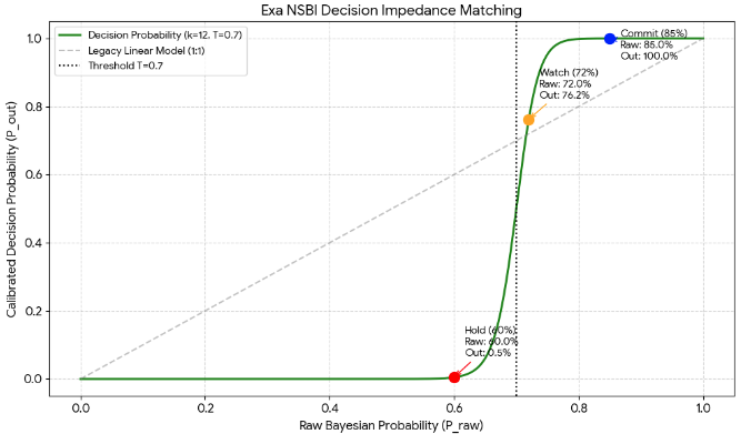
Let's prove how this mathematical model generates 'decision-making energy' through a real-world business scenario. Suppose we set the master reference values according to a certain organization's tendencies as follows:
- Decision-Making Threshold (): 0.7 (70%) - Interpretation: "There must be at least a 70% probabilistic basis to justify taking a gamble."
- Decision Acceleration (): 10 - Interpretation: "Act aggressively once the threshold is crossed."
Final Formula:
5.1 Business Scenario Simulation
Now, consider a stage in a sales negotiation process where the initial belief (prior distribution) has been sequentially updated to a posterior distribution. The α and β below are the values updated by the Bayesian engine from the negotiation stages and signals captured so far.
Situation 1: Below Threshold (A State of Hesitation)
- Data: (Pure Probability )
- Calculation Process:
- Ratio Calculation:
- Applying Power :
- Final:
- Interpretation: While the Bayesian probability is 60%, it falls short of the organizational threshold ( of 70%). The system cuts off the decision-making energy, sending a restrictive signal to the decision-maker: "Do not trust this yet (Hold)."
Situation 2: Threshold Breakthrough (Beginning of Decision)
- Data: (Pure Probability )
- Calculation Process:
- Ratio Calculation:
- Applying Power :
- Final Probability:
- Interpretation: As the probability slightly exceeds the threshold (T=0.7), the suppressed energy is released, and the pure probability begins to reflect directly on the dashboard. This is a signal that "it is now worth watching with interest (Watch)."
Situation 3: Critical Mass Breakthrough (Conviction Stage)
- Data: (Pure Probability )
- Calculation Process:
- Ratio Calculation:
- Applying Power :
- Final Probability:
- Interpretation: When the probability reaches 85%, the acceleration performs its magic. The system pushes the 85% figure into a 99.9% conviction (Commit) that "this project is a winning deal." The leader no longer has any reason to hesitate.
5.2 Insight Table
| Status | Pure Probability () | Calibrated Probability () | Decision Grade | Business Action |
|---|---|---|---|---|
| Below | 60% | 1.2% | Hold | Strictly prohibit resource input |
| Breakthrough | 72% | 72.4% | Watch | Begin strategic focus |
| Explosion | 85% | 99.9% | Commit | All-out resource concentration |
Insight: Why This Model Wins—The Systematization of Sales Decision-Making
- Elimination of False Hope: By decisively relegating deals with a 60% probability to a 1% level, the system inherently blocks 'unfounded optimism,' a chronic ailment in sales environments. Nevertheless, the 60% posterior probability remains important. Therefore, the engine must display both the Bayesian probability and the decision-calibrated probability together on the dashboard.
- Concentration on Bottleneck Resources: 72% and 85% are separated by only a 13% difference, but the system distinguishes them into entirely different dimensions of 'Interest' and 'Conviction.' Consequently, management instinctively knows which business to dedicate their time to.
- The Reality of Impedance Matching: This non-linear leap is a mathematical replica of the psychological state where veteran leaders feel, "I've got a gut feeling!" on the ground.
The power of the Bayesian engine lies not only in the logic itself but also in its flexibility to be tuned according to an organization's strategy and character.
Bayesian EXAWin-Rate Forecaster
Precisely predict sales success by real-time Bayesian updates of subtle signals from every negotiation. With EXAWin, sales evolves from intuition into the ultimate data science.