

This is the second commentary following Episode 1 of the EXA Manufacturing Operations Series, “The Idle Five-Axis Machine and the Mirage in the Conference Room.” In the factory portrayed in the story, every department was busy and pallets waiting to be machined filled the aisles, yet the parts needed that week did not reach the shipping area. While the first commentary examined each department's decision criteria, this article examines the physical consequences those decisions produced on the factory floor. The sales director cited high utilization to argue for more equipment, and Martin released materials earlier after a previous delay. Processing times and average capacity alone cannot establish when those decisions are appropriate and when they are not. Waiting at a shared resource depends not only on average load but also on variability in the intervals between arrivals and in processing times, and on the sequence in which jobs are processed.
This article uses queueing theory and Little's Law to explain the conditions under which work in process and waiting increase. Its purpose is to use that explanation to establish criteria for distinguishing problems that call for more equipment from those that call for changes to release and sequencing rules. It also examines why not all waiting is waste.
Rather than stopping at an introduction to theory, this article uses theory to explain what happened in the fictional factory. Adding capacity at busy equipment and releasing materials earlier are among the first responses considered on the shop floor when deadlines are at risk. The story showed work in process accumulating after early release and raised the possibility that adding equipment could increase waiting at other operations. This article examines those scenes through five questions.
- Why did production on the five-axis machine stop while a single first article waited at the measurement room (Section 1)?
- If the measurement room looked busiest, why were the five-axis machines the factory's bottleneck? Why did the manifolds wait behind boxes of covers whose due date was two weeks away (Section 2)?
- After Martin released materials earlier, pallets filled the aisles. Why were orders not completed sooner (Section 3, Little's Law)?
- What effect could the additional five-axis machine requested by the sales director on the basis of 95% utilization have on waiting at the measurement room (Section 4, Kingman's approximation in queueing theory)?
- Five weeks later, the parts on the staging shelf ahead of the five-axis machines were work in process, just like the pallets that had filled the aisles. What was different? When should idle time and waiting before an operation be reduced, and when do they provide necessary slack (Section 5)?
We examine these questions through task dependencies, release and processing sequences, and variability, as well as processing times.
Understanding the principles in detail by following the calculations requires close reading. On a first reading, it is also fine to focus on the situations compared in the tables and diagrams and on each section's interpretation and conclusions. The educational examples have been recalculated under their stated assumptions and checked against the figures in the tables and diagrams. Numbers quoted from the story are distinguished from assumptions made for the examples. Even without reproducing every calculation, readers can follow the argument by concentrating on what changes and what stays the same in each comparison.
The numerical examples in this commentary are educational models constructed to explain the principles, not measurements from the fictional factory. Whenever figures are taken from the story, their source chapter is identified.
1. The Dependency Between First-Article Approval and Production Machining
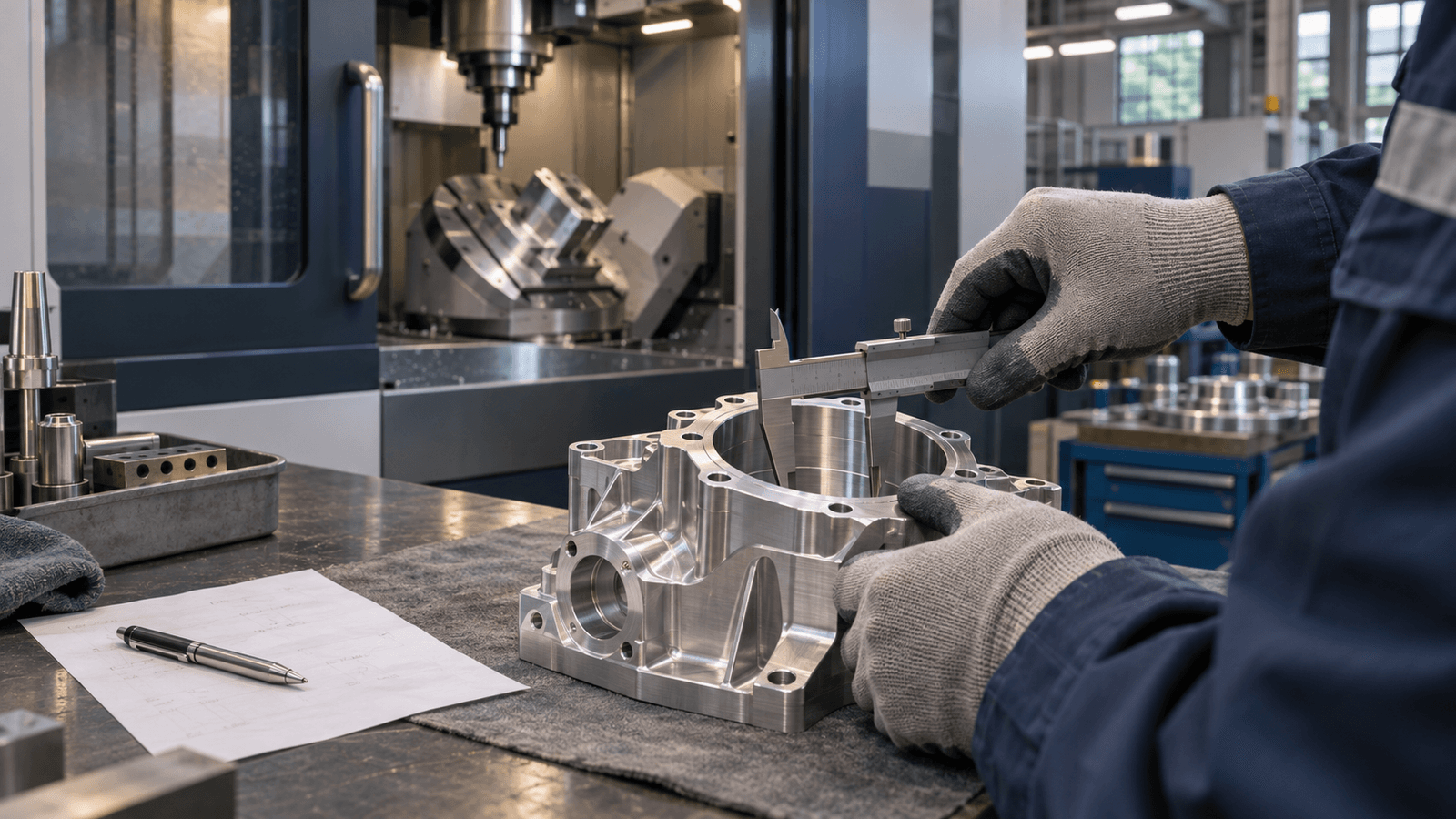
On Monday morning in Episode 1, five-axis Machine 1 had been idle for two hours. The first housing machined early that morning had gone to the measurement room, and the remaining 119 could not be machined until its dimensions were approved as conforming to the drawing. The measurement itself required only 15 minutes. But the measurement room's single CMM was measuring the parts that had arrived first from Line 3's lot of 300 brackets, in order of receipt.
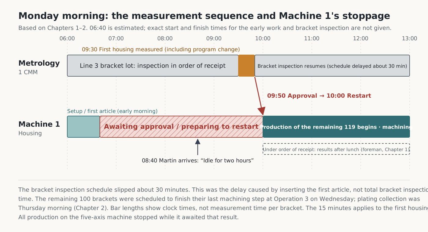
Two kinds of time separate in this scene. One is the processing time needed to do the job itself; the other is the waiting time before it can start. Processing time depends on such factors as geometry, process conditions, and the condition of equipment and tools. Waiting time depends on the amount and sequence of other work sharing the same resource, and on variability in that work. The first article's wait did not stay within the measurement room. While it awaited approval, production machining on five-axis Machine 1 also stopped. The measurement room and the five-axis machine were separate resources, but first-article approval connected them.
The same dependency appeared in the previous month's records for all three five-axis machines. At the meeting in Chapter 5, Martin broke down their controller records into the states making up a 24-hour day.
| Daily states of the three five-axis machines in the previous month (Chapter 5) | Time | Nature of the activity |
|---|---|---|
| Actual cutting | 9 hours | Machining |
| Tool and fixture changes (setup) | 4 hours | Preparation associated with machining |
| Waiting for first-article measurement results | 5 hours | Stopped because the approval condition had not been met |
| Waiting for material from an upstream operation | 6 hours | Stopped because parts had not arrived from the upstream operation: Operation 1 for the housings, Operation 3 for the manifolds |
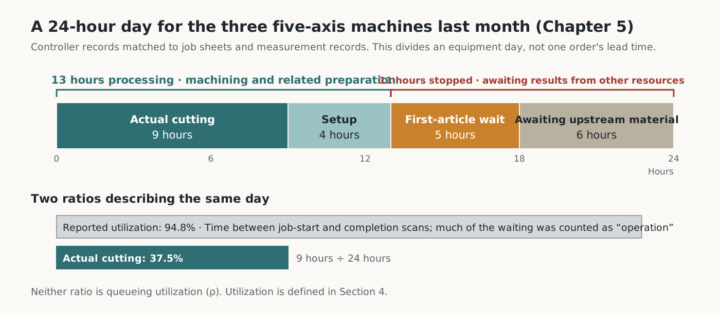
The report's utilization figure of 94.8% counted the time between the job-start and job-completion barcode scans. The proportion spent actually cutting was 37.5%. Even including setup as processing, the five-axis machines processed work for 13 hours a day; the remaining 11 hours were stoppages caused by results not arriving from other resources. This breakdown describes an equipment day, not the lead time of an individual order. Neither 94.8% nor 37.5% is utilization as defined in queueing theory. The 94.8% figure counted stoppages between barcode scans as operating time, while 37.5% counted only cutting. Queueing utilization is the proportion of time a resource spends processing arriving work. Its definition and the queueing formula are discussed in Section 4.
These figures contain a contrast. In Chapter 5, after rescheduling that week's confirmed orders operation by operation, Martin judged that the five-axis machines had the greatest capacity shortfall relative to the machining time required. Both Meriden parts had to pass through five-axis machining, and actual cutting times for both were longer than the standard times. Yet in the previous month those same machines had stopped for 11 hours a day because of the measurement room and upstream operations.
Even at the equipment with the greatest capacity shortfall, time not connected to upstream work and approval procedures could not be used for machining. This contrast is the starting point for answering the question carried over from Commentary 1: why the five-axis machines were the bottleneck, and how waiting built up ahead of them. The machining time available at the five-axis machines, which limited the factory's overall output, depended on sequencing and variability at other resources.
This is why the article turns to queueing theory. The story contains several decisions about waiting. Martin confirmed Meriden's deadline using the previous month's standard times and utilization report. The sales director cited 95% utilization to argue for buying another five-axis machine. After the prototype delivery was late, Martin extended standard lead times and released materials earlier to allow time to recover from delays. The measurement room followed the order of receipt so as not to favor any line.
Each decision had a rationale from its own perspective, but what remained in the factory was work in process filling the aisles and orders running late. Processing time and average capacity alone cannot adequately explain waiting at shared resources. Even resources with the same capacity can have different waiting times, depending on when jobs arrive, their processing sequence, and variability in their processing times.
Queueing theory separates waiting into job arrivals, resource processing, the service sequence, and variability. This separation makes it possible to ask whether an order is late because equipment capacity is insufficient, because release and sequencing rules created waiting, or because there was no allowance for variability. The article uses this theory to revisit three judgments.
First, how does the sequence of jobs sharing a resource affect waiting and due-date performance (Section 2)? Second, does earlier release bring completion forward (Section 3, Little's Law)? Third, why does waiting at a busy resource grow faster than its load, and what does that imply for capacity expansion and slack (Section 4, utilization and Kingman's approximation in queueing theory)?
Section 2 introduces the elements of queueing theory by mapping them to the measurement room; Section 4 presents the formula. Little's Law comes first, in Section 3, because it holds without assuming particular distributions for job arrivals or processing.
Building on those three answers, Section 5 examines why not all waiting is waste: some slack is deliberately maintained ahead of the bottleneck.
2. Waiting at Shared Resources and Job Sequencing
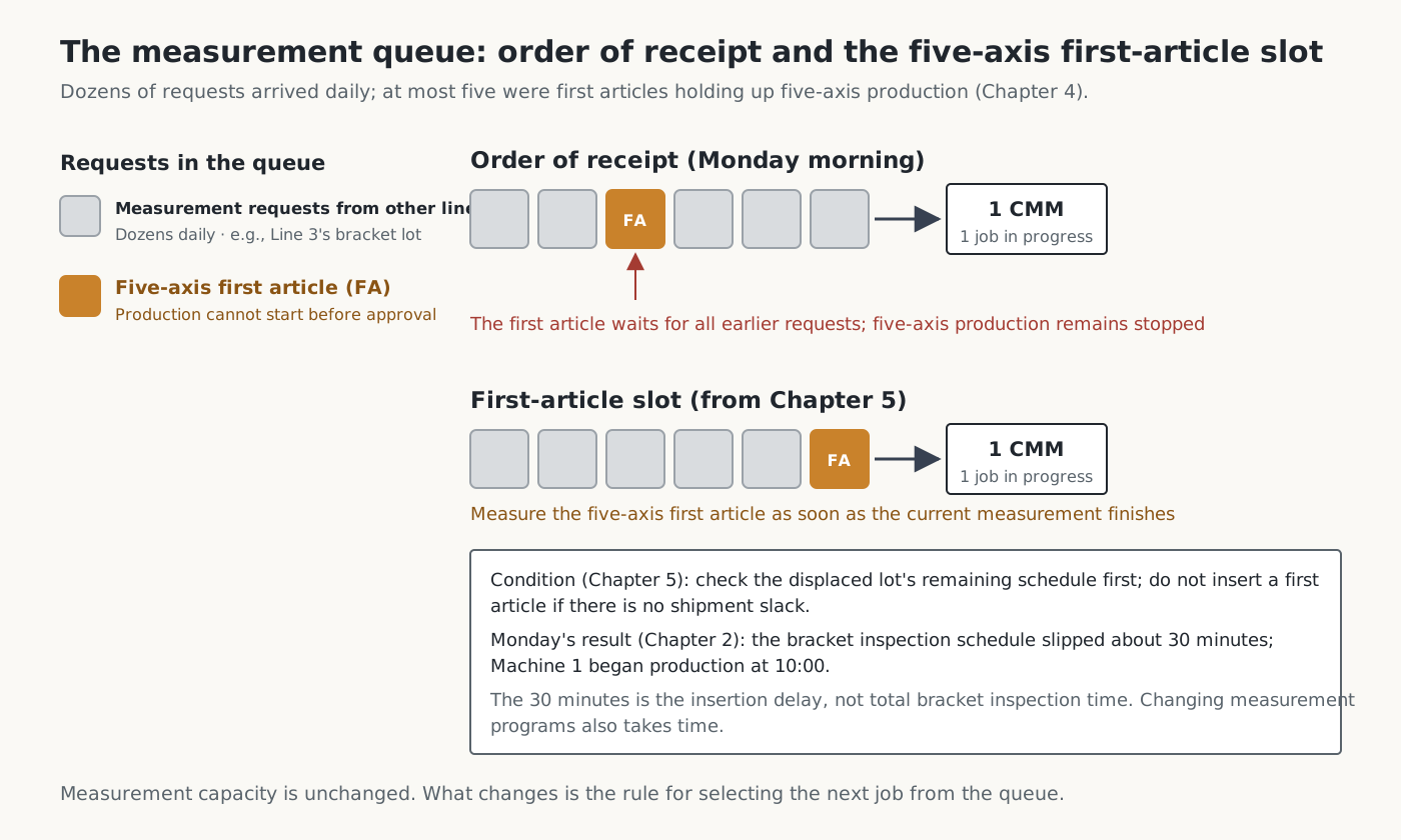
The measurement room was a shared resource serving several lines. It received dozens of measurement requests a day, at most five of which were first articles holding up five-axis machining. It processed requests in order of receipt (first-come, first-served). As the inspector explained, the measurement room could not tell which first article was stopping a five-axis machine. Order of receipt was a fair rule that favored no line, but it did not account for what else stopped while a part waited to be measured.
Queueing theory describes such a situation through several elements: how jobs arrive, how long the resource takes to process them, the rule for choosing the next job from the queue, and variability in arrivals and processing. This section focuses on the next-job rule; Section 4 uses a formula to examine how variability increases waiting. Applied to the measurement room, the elements are as follows.
| Element | In the measurement room |
|---|---|
| Arrivals | Measurement requests come from several lines. The inspector said there were dozens a day (Chapter 4). The number of requests must be distinguished from the number of parts to be inspected |
| Processing | Measurement on one CMM. Measuring the first housing took 15 minutes. The story does not give the actual number of brackets inspected or the time needed to measure them |
| Queue discipline | Order of receipt |
| Variability | Differences in the timing of request surges and in measurement times. The story does not give their distributions |
The “five-axis first-article slot” in Chapter 5 changed the queue discipline. The measurement room's capacity remained the same. The sequence changed. Once the measurement in progress finished, the five-axis first article would be measured ahead of other requests that had entered the queue earlier.
The items requiring inspection remain the same, but changing the sequence changes both first-article approval time and the schedules of other lots. Preparation needed for the change, such as switching the measurement program, must also be considered. In Chapter 2, measuring the first housing earlier pushed the bracket lot's inspection schedule back by about 30 minutes. These 30 minutes were the delay caused by inserting the first article, not the total time required to inspect the brackets. The brackets were scheduled to go to the plating supplier on Thursday morning, so the measurement room judged that the delay would not affect shipment. Had the first housing waited for those same 30 minutes, five-axis machining would have remained stopped for that much longer.
Martin attached a condition to the sequence change: check the remaining schedule of the affected lot before inserting a first article, and do not insert it if the lot has no slack.
This raises a question. The measurement room looked like the busiest place in the story. The probe kept moving without a break (Chapter 1), dozens of requests a day waited in order of receipt, and one sequence change immediately drew objections from another line (Chapter 8). Readers with production experience would suspect the measurement room before the five-axis machines as the bottleneck.
But the bottleneck is not simply the resource that looks busiest. A long queue and frequent complaints signal congestion at that resource. As Section 4 shows, queue length depends on variability in arrivals and processing and on the queue discipline, as well as on load. To identify the bottleneck, we must ask which resource still has the greatest capacity shortfall relative to the time needed to process confirmed orders after coordinating resources and schedules.
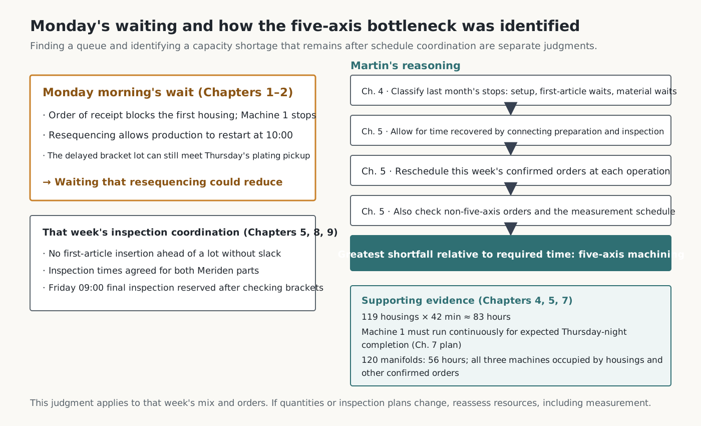
Martin did not identify the five-axis machines as the bottleneck immediately after finding the queue at the measurement room. In Chapter 4, he, the foreman, and the inspector separated five-axis stoppages into setup, waiting for first-article measurements, and waiting for material from upstream operations. In Chapter 5, he allowed for time that could be recovered by connecting preparation and inspection, then placed that week's confirmed orders back on the calendar operation by operation. He also checked orders that did not use five-axis machining and the measurement room's schedule separately. Even after that, the five-axis machines had the greatest shortfall relative to the time required.
The cause of Monday's waiting and the capacity shortage remaining after that cause had been addressed are separate judgments. The story does not show the underlying calculation in detail, and this commentary does not reproduce it. What is clear is that this judgment is part of the story's premise and that it was reached after checking the measurement room.
The five-axis shortage also appears elsewhere in the story. At 42 minutes each, the remaining 119 housings required about 83 hours (Chapter 4), and the schedule required Machine 1 to run without stopping to finish machining on Thursday night (Chapter 7). The 120 manifolds required 56 hours on Machine 2, but all three five-axis machines were occupied by housings and confirmed orders for other customers. Clearing Machine 2, splitting the work across openings on Machine 3, and outsourcing were all considered, but none allowed the manifolds to ship on Friday while honoring the other commitments (Chapter 5). The time at which roughing finished at Operation 3 also affected the manifolds' shipment date, so this outcome cannot be treated as evidence about the five-axis machines alone.
By contrast, the measurement room's schedule was coordinated around that week's orders. In Chapter 2, inserting the first housing delayed the bracket lot's inspection by about 30 minutes. The remaining 100 brackets were scheduled to finish their last machining step at Operation 3 on Wednesday, and collection for plating was on Thursday morning. In Chapter 5, Martin stipulated that first articles must not be inserted ahead of a lot with no slack before shipment. In Chapter 8, the measurement room agreed to perform intermediate and final inspections of the two Meriden parts at specified times. In Chapter 9, when the final housing measurement was moved to Friday morning, the quality manager checked the brackets' schedule before reserving the time. These scenes do not show that the measurement room had ample spare capacity. They show that inspection times could be coordinated with machining schedules for that week's product mix and due dates.
Thus, the story's premise in making five-axis machining the bottleneck is not that the measurement room was idle. It is the judgment in Chapter 5 that, even with inspection schedules coordinated, five-axis machining had the greatest capacity shortfall for that week's orders. On Monday, housing production stood still awaiting measurement-room approval, and changing the order of receipt could reduce that wait. The shortage of five-axis machining time could not be resolved solely by changing the measurement room's sequence.
The objections from other lines can be read in the same context. The quality manager worried that a resequenced lot might miss shipment (Chapter 5), while the bracket machining team asked why its inspections had been pushed back (Chapter 8). Both objections concerned inspection order and shipment schedules. Order of receipt was a fair rule that avoided such objections.
It did not, however, reflect which request was preventing a machine from processing work and which still had slack before shipment.
From a process-management perspective, recurring stoppages for approval should not be accepted as normal either. The housing could not enter production without the measurement room's approval. Concentricity tolerances on the order of five microns and three-dimensional free-form surface tolerances could not be judged from basic on-machine measurement data; machining expensive titanium without approval risked substantial losses if parts were defective (Chapter 1). Waiting for approval on such parts should be reduced by coordinating inspection capacity, schedules, and approval procedures with the machining schedule.
This judgment applies to that week's product mix and order conditions. If subsequent production quantities, lot composition, or inspection plans increase the work time required in the measurement room, the load and capacity of each resource, including the measurement room, must be checked again. Section 4 addresses those conditions.
The effect of sequence on due-date performance also appeared with the manifolds in Chapter 3. Their material had already been released to the floor, but it sat ahead of the Operation 3 mill behind boxes of covers due two weeks later. The covers could be machined consecutively using the same fixture and program, and their release date had been brought forward. Release timing and a resource's processing sequence are separate decisions, but they become linked if work released first takes the first positions at a shared resource.
A simple example illustrates this structure. The numbers below are assumptions, not the actual processing times of the covers and manifolds. One machine has two later-due jobs, K1 and K2 (2 hours each, due at hour 8), and an urgent job U (1 hour, due at hour 3). K1 and K2 become available for processing at hour 0, and U at hour 1. Jobs are processed in release order, and once started, a job cannot be interrupted. Setup, transport, and switching between jobs take no time. This example does not reproduce the capacity of the actual measurement room or mill; it isolates the effect of sequence.
| Release rule | Processing intervals | U completion / lateness | K2 completion / lateness |
|---|---|---|---|
| Release jobs as soon as they are ready | K1 hours 0–2, K2 2–4, U 4–5 | Hour 5 / 2 hours | Hour 4 / None |
| Hold K2 until hour 3 | K1 hours 0–2, U 2–3, K2 3–5 | Hour 3 / None | Hour 5 / None |
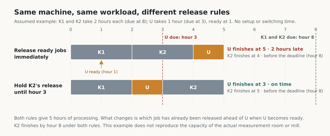
The machine processes work for the same total of 5 hours under both rules. What changes is what has already been released ahead of the urgent job when it reaches the shared resource. Real factories have setups and downstream operations, so this example does not establish whether the manifolds could have shipped on Friday.
3. Work in Process, Throughput Rate, and Flow Time — Little's Law
After a previous delay, Martin extended standard lead times and released materials earlier to create time for recovery. To determine whether earlier release brings completion forward by the same amount and creates recovery time, we need to understand the average relationship among work in process, throughput rate, and flow time inside the factory.
This section first establishes that relationship, then compares examples in which only the release pattern changes while other conditions remain the same. The pallets filling the aisles are work in process (WIP). Little's Law describes what changes along with work in process inside the factory. Proven by John D. C. Little in 1961, it relates three averages: the average work in process within a boundary, the average throughput rate across that boundary, and the average time a job spends inside it. The boundary defines the scope within which work and time are counted. It can encompass the whole factory, a single operation, or a measurement room.
Let us unpack the formula.
- L is the average number of jobs within the boundary during the observation period, measured in jobs. It counts both jobs being processed and jobs waiting. For each interval during which the job count is constant, multiply the count by the interval's duration. Add those products and divide by total observation time. The numerator is measured in job-hours, so dividing by hours leaves jobs.
- λ is the average throughput rate: the number of jobs completed during the observation period divided by total observation time. Its unit is jobs per hour. This rate measures physical volume and is different from the monetary measure T in the throughput accounting discussed in Commentary 1.
- W is average flow time: add up the time each job spends between entering and leaving the boundary, then divide by the number of jobs. It includes processing time and waiting time within the boundary and is measured in hours. In this article's examples, it is the average lead time from factory release to completion.
Calculating all three for a simple two-job example makes the distinction clear. Jobs A and B enter an empty workshop together at 09:00. There is one machine, and each job requires 1 hour of processing. A is processed first and leaves at 10:00; B follows and leaves at 11:00. The observation period runs from their arrival at 09:00 until both have left at 11:00, a total of 2 hours.
| Interval | Job A | Job B | Jobs inside |
|---|---|---|---|
| 09:00–10:00 (1 h) | Processing | Waiting | 2 jobs |
| 10:00–11:00 (1 h) | Completed; left | Processing | 1 job |
L is the average number of jobs inside the workshop over the 2 observed hours. There are 2 jobs during the first hour and 1 during the next. Thus L = (2 jobs × 1 hour + 1 job × 1 hour) ÷ 2 hours = 1.5 jobs. B counts as work in process during its first hour of waiting because it is inside the workshop. This does not mean that there were 1.5 jobs at any particular moment. The average weights the count in each interval by how long that interval lasts. Here, both intervals last 1 hour, so the result equals the simple average; unequal intervals must be weighted by their durations.
λ indicates the average number of completions per hour. During the 2 observed hours, A and B are completed: 2 jobs in total. Therefore λ = 2 jobs ÷ 2 hours = 1 job per hour.
W is the average time a job spends between entering and leaving. A enters at 09:00 and leaves at 10:00, spending 1 hour inside. B enters at 09:00 and leaves at 11:00, spending 2 hours inside. Thus W = (1 hour + 2 hours) ÷ 2 = 1.5 hours. B's 2 hours include both 1 hour of waiting and 1 hour of processing.
Substituting these values into Little's Law gives 1.5 jobs = 1 job per hour × 1.5 hours. L is the average number of jobs inside the workshop, λ the average completions per hour, and W the average flow time per job.
The three values must refer to the same process boundary and observation period. Use one consistent counting unit, such as jobs or pieces, and one time unit, such as hours or minutes. L, λ, and W themselves have different units: jobs, jobs per hour, and hours. If there are no jobs within the boundary at the beginning and end of observation, the formula holds exactly for that period's records. It may not match if jobs entered before observation began or remain after it ends. In that case, specify whether those jobs are included in or excluded from the calculation.
The formula also states only that the three averages must be consistent; it does not identify which is the cause. An increase in work in process implies a longer flow time only when throughput rate does not increase further. For example, if the completion rate remains fixed by bottleneck capacity, putting more jobs into the factory only increases how long each waits. If throughput rate can increase as well, work in process may rise while flow time remains unchanged.
The next example examines this relationship. Operations P and Q are connected in series, with one machine at each operation. P takes 1 hour per job and Q takes 2 hours. P plays the role of an upstream operation and Q the bottleneck, but the figures are unrelated to the story. Jobs J1–J4 all exist as orders at hour 0, and their materials are ready. Their due dates are hours 4, 6, 8, and 10, respectively, and they are processed in the order J1 through J4. Assume no setup, transport, inspection, or defects. The boundary runs from release to P through completion of processing at Q, and the observation period is hours 0–12. There is no work in process within the boundary at the beginning or end of this interval.
We compare two release patterns. Simultaneous release puts all four jobs into the factory at hour 0. Paced release introduces one job at hours 0, 2, 4, and 6, matching Q's processing interval.
| Job | Simultaneous release: P interval / Q interval | Paced release: release / P interval / Q interval |
|---|---|---|
| J1 | 0–1 / 1–3 | 0 / 0–1 / 1–3 |
| J2 | 1–2 / 3–5 | 2 / 2–3 / 3–5 |
| J3 | 2–3 / 5–7 | 4 / 4–5 / 5–7 |
| J4 | 3–4 / 7–9 | 6 / 6–7 / 7–9 |
| Observation: hours 0–12 | Simultaneous release | Paced release |
|---|---|---|
| Completion times | Hours 3, 5, 7, 9 | Hours 3, 5, 7, 9 |
| Completions / average throughput rate λ | 4 jobs / 1/3 job per hour | 4 jobs / 1/3 job per hour |
| Flow time by job | 3, 5, 7, 9 hours | 3, 3, 3, 3 hours |
| Average flow time W | 6 hours | 3 hours |
| Average WIP L | 2 jobs | 1 job |
| Lateness | None | None |
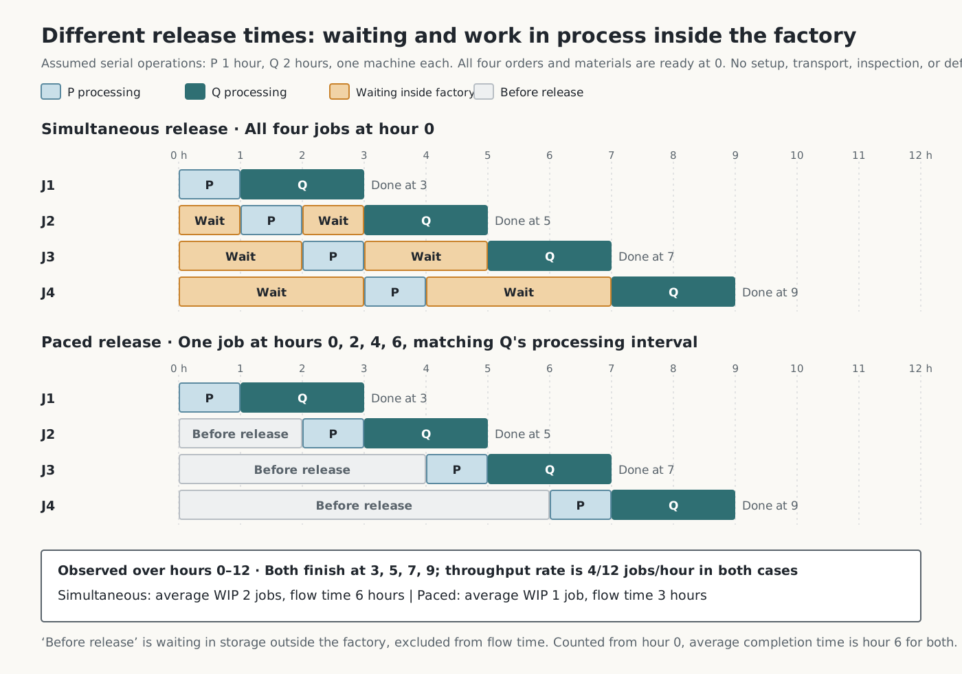
To calculate average WIP L under simultaneous release, first determine how many jobs are inside the factory during each part of the 12-hour observation period. All four enter at hour 0, and one finishes and leaves at each of hours 3, 5, 7, and 9.
| Interval | Jobs within the boundary | Duration | Job count × duration |
|---|---|---|---|
| Hours 0–3 | 4 jobs | 3 hours | 12 job-hours |
| Hours 3–5 | 3 jobs | 2 hours | 6 job-hours |
| Hours 5–7 | 2 jobs | 2 hours | 4 job-hours |
| Hours 7–9 | 1 job | 2 hours | 2 job-hours |
| Hours 9–12 | 0 jobs | 3 hours | 0 job-hours |
| Total | — | 12 hours | 24 job-hours |
Average WIP is therefore 24 job-hours ÷ 12 hours = 2 jobs. “Time average” does not mean averaging time. It means averaging a job count that changes over time, weighted by the duration of each interval.
Average flow time W is a different calculation. Add the four jobs' individual flow times of 3, 5, 7, and 9 hours, then divide by 4 jobs: (3+5+7+9) ÷ 4 = 6 hours. For average throughput rate λ, divide 4 completed jobs by the 12 observed hours: 4 jobs ÷ 12 hours = 1/3 job per hour.
The same method applies to paced release. There is 1 job within the boundary during hours 0–2, 2 during 2–3, 1 during 3–4, 2 during 4–5, 1 during 5–6, 2 during 6–7, 1 during 7–9, and 0 during 9–12. Multiplying each job count by its interval's duration and adding gives 12 job-hours. Dividing by 12 observed hours gives average WIP of 1 job. Each of the four jobs spends 3 hours inside, so average flow time is 3 hours. Completions remain at 4 jobs, so average throughput rate is also unchanged at 1/3 job per hour.
Both patterns satisfy Little's Law.
In this example, Q takes 2 hours per job, so its capacity when processing continuously is 1 job ÷ 2 hours = 0.5 job per hour. During the actual observation period, hours 0–12, it completes 4 jobs, for a throughput rate of 1/3 job per hour. The observation period includes hours 0–1 and 9–12, when Q does not process work, so this rate is lower than capacity.
Under both release patterns, Q processes continuously from hour 1 to hour 9, giving identical completion quantities and times. Simultaneous release does not bring completion forward; it only doubles work in process and flow time. With simultaneous release, a job waits an average of 1.5 hours before P and 1.5 hours before Q. With paced release, there is no waiting before either operation, reducing average flow time from 6 hours to 3 hours.
The example shows one further distinction. The 3-hour flow time under paced release is measured from release onward. It excludes the 0, 2, 4, and 6 hours the jobs wait in storage before release. Measured from order arrival at hour 0 through completion, both patterns take 3, 5, 7, and 9 hours, averaging 6 hours. The waiting removed from inside the factory under paced release has simply moved to time spent unreleased in storage. A reduction in work in process inside the factory therefore does not by itself mean a shorter wait for the customer.
In this example, earlier release leaves completion times unchanged; it merely moves waiting from before release into the process. Under a rule that processes earlier-released work first, as in Section 2, the work moved into the process also affects the machining sequence of other orders. Section 6 of Commentary 1 discusses how machining materials early limits the available paths for recovering their value.
4. How Utilization and Variability Increase Waiting — Queueing Theory and Kingman's Approximation
The example in Section 3 had no variation in processing times. In a real factory, jobs do not arrive at regular intervals, and processing times differ from job to job. This explains why waiting occurs even at a resource whose average capacity appears sufficient.
This section revisits two scenes in the story: the request to buy another five-axis machine on the basis of reported utilization, and the long queue at the measurement room, which looked busiest. Understanding how utilization and variability increase waiting helps avoid concluding that capacity is insufficient merely because a queue is long. It also helps anticipate how rapidly waiting can grow when more work is assigned to an already busy resource.
Queueing theory includes various models of arrivals and processing. The well-known M/M/1 model describes a system with one machine, where the number of jobs arriving in a given period follows a Poisson distribution and interarrival times and processing times each follow an exponential distribution. The Poisson distribution describes the “number” of arrivals in a period; the exponential distribution describes the “time interval” until the next arrival. Not all queueing models assume Poisson arrivals, however. Kingman's approximation in this section does not fix interarrival and processing times to one particular distribution; it uses their respective means and variability.
Here, λ is the average arrival rate: the number of jobs arriving at a resource per unit of time. Section 3 used the same symbol for the average throughput rate of completed jobs. In a stable system where jobs do not disappear or leave midway and the queue does not keep growing, long-run average arrival and throughput rates are equal. That does not mean arrivals and completions are always equal over a short observation interval.
This section assumes one machine that processes whenever work is available, with no breakdowns or shift interruptions. Under these conditions, utilization ρ is the long-run proportion of time spent processing, calculated by multiplying average arrival rate by average processing time per job. For example, if an average of 4.8 jobs arrive per hour and each takes an average of 10 minutes, the work arriving each hour requires an average of 48 processing minutes. Utilization is 48 minutes ÷ 60 minutes = 0.8, or 80%. Average waiting time at one resource can be estimated with Kingman's approximation.
Let us unpack the formula.
- E[ ] denotes the mean of the value inside the brackets. E[S] is average processing time per job, measured in minutes in the example below.
- E[W_q] is the average time a job waits between arrival and the start of processing, measured in minutes. It excludes processing time. To obtain average flow time at this one machine, add E[S] to E[W_q].
- c_a² is the standard deviation of interarrival times divided by their mean, then squared. c_s² applies the same calculation to processing times. Standard deviation describes how widely values are dispersed around their mean. For example, if mean processing time is 10 minutes and standard deviation is 5 minutes, c_s² = (5 minutes ÷ 10 minutes)² = 0.25. Both quantities are dimensionless because the same time units cancel. Larger values mean greater variability relative to the mean.
- The first factor represents variability, the second the effect of utilization, and the third the scale of processing time. Average waiting is approximated by the product of these three factors.
The variability and utilization factors are dimensionless, so multiplying them by average processing time gives a result in units of time. Entering processing time in minutes produces average waiting in minutes.
The second factor, ρ/(1−ρ), grows much faster than utilization. It equals 1 at utilization of 0.5, but 4 at 0.8, 9 at 0.9, and 19 at 0.95. With average processing time and variability held constant, utilization increases by less than a factor of two from 0.5 to 0.95, while the approximation's average waiting time increases nineteenfold. The first factor shows that, at the same utilization, waiting is longer at resources with greater variability.
The table below compares two variability conditions with average processing time set to 10 minutes. The variability factor is the first factor, (c_a²+c_s²)/2. A factor of 0.5 represents a case where the squared coefficients of variation of both interarrival and processing times are 0.5: arrivals are relatively even and processing times do not vary greatly. A factor of 2 represents values of 1 and 3, respectively: jobs arrive randomly and processing times vary considerably from job to job. These are all assumed values.
| Utilization ρ | Average waiting (variability factor 0.5) | Average waiting (variability factor 2) |
|---|---|---|
| 0.60 | 7.5 minutes | 30 minutes |
| 0.80 | 20 minutes | 80 minutes |
| 0.90 | 45 minutes | 180 minutes |
| 0.95 | 95 minutes | 380 minutes |
Under the first condition, at utilization of 0.8, average waiting is 0.5 × (0.8 ÷ 0.2) × 10 minutes = 20 minutes. The 10 minutes of processing are separate, so average flow time from arrival to completion is 20 minutes + 10 minutes = 30 minutes.
This approximation concerns long-run averages in a model where one machine processes jobs to completion in order of receipt; interarrival times are independent draws from one common distribution; processing times are independent draws from a separate common distribution; and interarrival and processing times are mutually independent. Utilization must also be below 1, so that average load does not exceed capacity.
This one formula cannot predict a real factory with setups, breakdowns, approvals on hold, shift interruptions, and intertwined routing. The utilization of 0.95 in the table is also different from the 95% reported in the story, and average waiting does not indicate the probability that a particular order will be late. The formula provides direction: as utilization of a shared resource approaches 1, and as variability in arrivals and processing increases, waiting grows much faster than load.
The table is a calculation for a hypothetical resource, not a specific machine, and does not describe the measurement room's load in the story. The story does not specify the scope or time of bracket inspection or the measurement room's available time. Its figures therefore cannot establish whether the entire inspection schedule is feasible or what the measurement room's actual utilization is. What the story does establish is the dependency by which first-article approval was blocking five-axis machining, and the fact that order of receipt affected that wait. The judgment that the measurement room was not that week's bottleneck was not derived from a utilization figure either. As Section 2 showed, it rests on the judgment in Chapter 5 that five-axis capacity remained most insufficient after coordinating inspection schedules, together with the scenes in which the measurement schedule was adjusted. How much variability increases when jobs with different processing times are mixed depends on their individual times and proportions in the mix. With mean processing time, utilization, and interarrival variability held constant, greater processing-time variability produces longer average waiting in the approximation above. The story lacks the data needed for this comparison, so actual waiting at the measurement room cannot be calculated.
In Chapter 5, Martin reported that adding another five-axis machine would also increase the time spent waiting for first articles at the measurement room and for roughing. The approximation shows the conditions on which that claim depends. If expansion increases actual production volume or the number of lots, resulting in more first-article and intermediate inspection requests to the same measurement room, while its available time and processing conditions remain unchanged, its load rises. If utilization is already high, even a small increase in load can cause a much larger increase in waiting. However, the story does not provide the data needed to calculate measurement-room utilization, so this article does not quantify the increase in waiting. Nor does the approximation prove that adding equipment would fail to increase production. Commentary 1 discusses the criteria for evaluating expansion; Commentary 4 will examine capacity judgments once records have accumulated.
5. Repeated Early Release and Protecting the Bottleneck
In Chapter 3, Martin recalled that delivery of the Meriden prototypes had been ten days late. Concluding that work had started too late, he extended standard lead times for Meriden parts, then applied the same approach to other orders. Standard lead time is the duration a scheduling system subtracts from the due date to set the release date. Extending it brought materials for several orders onto the floor earlier.
Combining the early release and waiting observed in the story with a hypothesis about repeating the same response gives the following cycle.
Late prototype delivery
  → Longer standard lead time → Earlier release of multiple orders
  → More shop-floor WIP → More waiting at shared resources → Longer actual flow time
  → Lead time appears insufficient → (If the same response is repeated) Further extension of standard lead time
According to Little's Law, when two states have the same throughput rate, higher average work in process means longer average flow time. If that result is attributed to late release and release is brought forward again, the same waiting may recur. Martin reconsidered this judgment explicitly at the Chapter 5 meeting: by putting “recovery time at the very beginning,” he had turned that time into pallets filling the aisles.
This cycle is, however, a causal hypothesis to examine in this factory. It does not explain delays at every factory by the same cause. Other causes overlapped in this case as well. As Chapter 4 established, actual cutting times for both Meriden parts exceeded the standard times in the master data. Actual capacity shortages must be distinguished from waiting created by operating policy.
Batch processing fits into the same structure. Machining the covers consecutively with the same fixture was a rational way to reduce setups. As the foreman said, splitting the batch midway would require another setup later. Yet other jobs needing that machine must wait until the batch ends. Setup savings and waiting for other jobs are a trade-off. Martin and the foreman's decision to finish only the batch in progress and hold the remaining covers reassessed that trade-off against the manifolds' due date.
Adding one delay to the Section 3 example shows whether reducing work in process is sufficient on its own. Suppose J3's processing time at P increases from 1 hour to 3 hours. Apply the same delay to both release patterns, without changing release times after observing it. Add a third pattern in which only some jobs are released ahead of time: at hours 0, 0, 2, and 4. The preparation allowance is the time parts that have completed the upstream operation wait for their turn at Q. Without the delay, this pattern provides allowances of 0, 1, 2, and 2 hours for J1 through J4.
| When J3 takes 3 hours at P | Simultaneous release (hours 0, 0, 0, 0) | Paced release (hours 0, 2, 4, 6) | Selective early release (hours 0, 0, 2, 4) |
|---|---|---|---|
| Completion times at Q | Hours 3, 5, 7, 9 | Hours 3, 5, 9, 11 | Hours 3, 5, 7, 9 |
| Average WIP | 2 jobs | 4/3 jobs (about 1.3) | 1.5 jobs |
| Lateness | None | 2 jobs, 2 hours in total | None |
| Time Q is idle for lack of work between its first start and final completion | None | 2 hours (hours 5–7) | None |
Paced release had the lowest work in process, but because no job was ready ahead of Q, a single upstream delay directly stopped the bottleneck. Those 2 hours of bottleneck stoppage translated into lateness for J3 and J4. Simultaneous release absorbed the delay but carried the most work in process. Selective early release absorbed the same delay with less work in process than simultaneous release. This result describes one delay scenario; it neither calculates the optimal allowance nor proves due-date reliability. A larger delay or a delay affecting a different job would change the outcome. In this scenario, preparing some jobs early maintained continuous processing at Q and on-time completion with less work in process than simultaneous release. Work in process prepared to be ready when needed can absorb upstream delays. Its effect depends on which jobs are ready, their sequence, and the size of the delay.
Chapter 11 presents this distinction in a scene. Five weeks later, parts that had completed upstream operations waited their turn on the staging shelf at the entrance to the five-axis area before moving to the machines. Both the pallets that filled the aisles and the parts on the shelf were waiting work in process. The former had been released before they were needed and had taken positions ahead of other orders. The latter provided a buffer so that upstream delays would not interrupt bottleneck machining. Even the same act of waiting has different effects on the factory depending on its location and quantity.
Spare capacity at non-bottleneck resources can be read in the same way. In the same Chapter 11, a general-purpose mill at Operation 3 stood idle, and no one pressured its operator. Commentary 1 read this scene as a change in evaluation rules. The formula in Section 4 shows that, at a resource with variability in arrivals and processing, pushing utilization close to 1 makes waiting grow much faster than utilization. If upstream operations are always fully loaded, they have no capacity left to catch up on delayed preparation and resupply the bottleneck. An empty slot on a calendar is not itself that capacity, however. The tools, people, and quality conditions needed during the slot must be in place for it to provide actual recovery capacity.
Commentary 3 will discuss how to size the preparation allowance ahead of the bottleneck, work backward from its schedule to set release times, and distinguish that allowance from time provided ahead of shipment.
6. The Records Five Weeks Later and the Work Still to Be Done
Five weeks later, the yellow safety lines were visible again in the aisle ahead of the five-axis area. Materials left storage only on dates calculated backward from the five-axis schedule by allowing the time needed for upstream operations. Setup time had fallen from 90 minutes to 25 minutes, and five-axis first articles seldom piled up at the measurement room anymore.
The scope of these results must also be stated. Improvements centered on the five-axis area, while boxes still filled aisles elsewhere. One shipment was half a day late despite the time allowed ahead of shipping. Martin's records still contained long lists of waits for first articles, tools, and materials. What changed was that each entry now had a cause and an owner. Alongside the total amount of waiting, the factory began to examine where it occurred, why it occurred, and which orders it delayed. These records do not provide a basis for calculating percentage improvements in factory-wide average work in process or flow time, and this article presents no such figures.
Applied to another factory, the same questions are as follows.
- Is stoppage time at key equipment recorded separately as setup, waiting for approval, and waiting for material? Does reported utilization distinguish those stoppages from operation?
- What is the utilization of resources shared by several lines, such as inspection, heat treatment, and painting, and what rules determine their queue order?
- Do those sequencing rules account for the machines that stop and the orders that run late while jobs wait?
- Is earlier release the default response when a deadline is at risk? How have shop-floor work in process and actual flow time changed in response?
- Where is the work in process that provides preparation allowance to protect the bottleneck, and where is the work in process that accumulated because it was released before it was needed?
The remaining questions lead to the next commentary: when should materials be released, and where and how much slack should be provided?
Next · Commentary 3. Synchronizing Production Planning and Execution
Martin decided to set the five-axis schedule first, then connect material, measurement, and shipment to it. The next commentary explains release paced to the bottleneck, externalizing setup work, and designing time allowances to protect shipment through the principles of finite-capacity scheduling and time buffer management.
Join the discussion