

Just when I thought the case was closed, I opened the records again.
The morning evidence pointed toward temperature. Five of 50 items were defective. The probability that temperature was the cause had risen to 87.6%.
But the afternoon record contained just one defective item out of 50. Confidence fell to 63.7%.
The number changed. The morning evidence did not disappear.
“If the afternoon had also produced five defects, would I have reached the same judgment?”
For a moment, I decided to become the investigator again.
Reopening the case
Part 1, The Silent Factory followed two suspects: temperature and pressure. Part 2, the mathematical explanation, opened up the calculation behind the changing judgment.
Now you can change the conditions of the same case yourself. The experiment below does not draw a random answer. It calculates how strongly your evidence supports each hypothesis and carries the result forward as the starting point for the next judgment.
Keep three ideas in mind: the prior is your initial belief, likelihood describes how well each cause explains this result, and the posterior is your judgment after accepting the evidence. A 60% cause probability and an 8% defect probability answer different questions.
Start with Original case. Before applying the morning evidence, predict which way the temperature probability will move. Then follow Investigation notes through “Likelihood → Evidence strength → Update.” On a wide screen the notes stay beside the article; on a smaller screen they continue below the experiment.
The notes combine the explanation needed at each stage with your actual numbers. Links open the relevant section of Part 2 in a new tab for the full derivation.
Change the numbers and run your own experiment. 60, 50, 5 and 1 are starting values. Click the prior, sample-size or defect-count field, enter your own number, then apply the evidence. Question buttons load examples; they do not restrict your inputs.
When evidence changes, judgment changes.
Predict, change the records, and explain why the result changes.
- 60% · Initial belief
- The share of past cases attributed to temperature. This is the prior belief for this case.
- 8% / 4% · Cause-specific rates
- Defect probability per item if temperature / pressure is the cause. These rates stay fixed.
- 5/50 → 1/50 · New evidence
- Five morning defects, then one defect in a new afternoon sample. The samples do not overlap.
H_T is the temperature hypothesis; H_P is the pressure hypothesis. 60% and 8% answer different questions.
Use a question button to load an example, or enter your own values. The question and inputs change with your selection. Apply the evidence to update both the results and the investigation notes.
Can temperature remain more likely even when afternoon evidence supports pressure?
See how morning's conclusion becomes afternoon's starting point.
An example is just a starting point. You can edit the numbers. Apply evidence again from the edited stage to update the results and investigation notes.
60, 50, 5 and 1 are starting values. Click the prior, sample-size or defect-count field, enter your own number, then apply the evidence. Question buttons load examples; they do not restrict your inputs.
Change the numbers and click “Apply evidence” to update the result. The case notes on the right show the formulas and calculation steps with your own numbers substituted. On smaller screens, find the case notes below.
Enter the sample size and observed defects for each new inspection. Causes and evidence are not generated randomly.
Why this calculation? · Open the investigation notes ↓Current judgment
Before inspection
Probability that pressure is the cause 40.0%
This is the prior judgment. Apply the morning record first.
Select a record to see its investigation notes. Green represents temperature; ochre represents pressure.
Compare with the original case
| Stage | Original case | My experiment |
|---|---|---|
| Before inspection | 60.0% | 60.0% |
| After Morning | 87.6% | Pending |
| After Afternoon | 63.7% | Pending |
The original case uses a 60% prior, 5/50 in the morning, and 1/50 in the afternoon. Compare these with your inputs.
Show the stage-by-stage table
| Stage | Defects / Inspected | BF | Temperature : Pressure odds | Temperature probability |
|---|---|---|---|---|
| Before inspection | — | — | 1.500000 : 1 | 60.0% |
We assume one of the two hypotheses is the cause, fixed defect rates of 8% and 4%, and independent inspections conditional on the cause. Results are relative cause probabilities under these assumptions. Revisit the model if equipment conditions or the cause change between inspections.
Three questions to continue the investigation
What if the afternoon also had five defects?
First apply the morning and afternoon evidence using the original values. The temperature-cause probability follows 60% → 87.6% → 63.7%.
Choose Question 1 · Five defects again in the afternoon. Keep the prior at 60% and the morning record at 5/50; change only the afternoon defect count from one to five. What happens when another sample points in the same direction as the morning evidence?
Read the explanation after experimenting
The temperature probability reaches about 97.1%. The morning and afternoon Bayes factors are both approximately 4.714. Applying two samples pointing in the same direction increases the temperature-to-pressure odds. Compare the stages under Evidence strength in the notes.
What if you suspected pressure more strongly at first?
Choose Question 2 · Start with a 30% prior. Restore the records to 5/50 in the morning and 1/50 in the afternoon, and change only the temperature prior from 60% to 30%.
The evidence is the same, but the starting point is different. Which quantities change, and which stay the same? In Investigation notes, the Bayes factors for the same records stay unchanged while the prior odds differ.
Read the explanation after experimenting
The path becomes 30% → 66.9% → 33.4%. Compare it with the original 60% → 87.6% → 63.7%. BF compares the evidence under the two hypotheses, so it stays the same. The starting point changed, and therefore so did the posterior.
What if there were no afternoon defects?
Choose Question 3 · Zero afternoon defects. Keep the 60% prior and morning 5/50; change only the afternoon to 0/50.
The absence of defects is evidence too. But this experiment compares the relative plausibility of two specified causes. A lower observed defect rate does not, by itself, establish that the underlying problem has disappeared.
Read the explanation after experimenting
The temperature probability falls from 87.6% after the morning inspection to about 45.7%. All 50 good items enter the likelihood, and this evidence favors pressure, the hypothesis with the lower defect rate. We did not calculate a third “healthy equipment” hypothesis, so this is not a conclusion that the cause has vanished.
Return to the experiment choices
Carrying forward the next lot's record
In Part 1, the engineer proposed taking another sample of 50 from the next lot. After the first two inspections, Add the next inspection lets you continue that scene yourself. The defect count is not predetermined. Enter a new record and see how the current conclusion becomes the next starting point.
Add only newly observed items each time. Entering the morning or afternoon record again would count the same evidence twice. More records do not necessarily increase confidence at every step. It can rise or fall with individual samples as evidence accumulates under the assumption of the same cause and defect rates.
Does calculating in stages give the same answer as pooling?
Use Compare sequential and pooled calculations to check the result from Part 2, Section 9. In the original case, updating twice with 50 items each or calculating once from six defects among 100 items gives the same temperature probability: about 63.7%.
These are two separate calculations from the same starting point. You are not adding the pooled 100 items to a judgment already updated twice. When inspection conditions stay fixed and observations are independent given the same cause, the product of the individual BFs equals the BF of the combined evidence.
Read why confidence changed, not just how large it is
A moving probability bar does not close the investigation.
You need to explain what evidence arrived, which hypothesis makes it more likely, and what it adds to the earlier judgment. Investigation notes show the Bayes factor and odds calculations using your inputs.
The experiment assumes either temperature or pressure is the cause, with defect probabilities fixed at 8% and 4%. If equipment conditions change between inspections or another cause intervenes, first revisit the model to account for that change.
Even when afternoon evidence supports pressure, temperature can remain more likely overall. The direction of this evidence and the judgment after all evidence so far are different questions. The afternoon update starts from what the morning evidence has already established.
Explain it in your own words: “Which cause did this evidence support? What did I carry forward? Why did the probability change?” A cause probability does not automatically decide whether to maintain or stop equipment. The next decision also considers inspection costs, shutdown costs, and the risk of defective items escaping.
Before closing the records, ask one last question.
“Am I protecting my initial conviction, or accepting the new evidence?”


Join the discussion